Tutorial — Manhattan Post-Event Traffic Management

This walkthrough reproduces the Manhattan post-event case study from the paper (Section 5.3.2): a city operator faces a concentrated departure surge from Madison Square Garden (MSG) into the surrounding network and asks AgentSUMO to compare two signal-control policies for mitigating it.

Unlike the Seoul tutorial, the user does not specify the intervention. The request only states the goal — “find where congestion builds up and how to clear it faster” — leaving the agent to formulate the problem, decompose it, and choose policies to compare. The IPP classifies this as an Agentic task, one step above Complex.

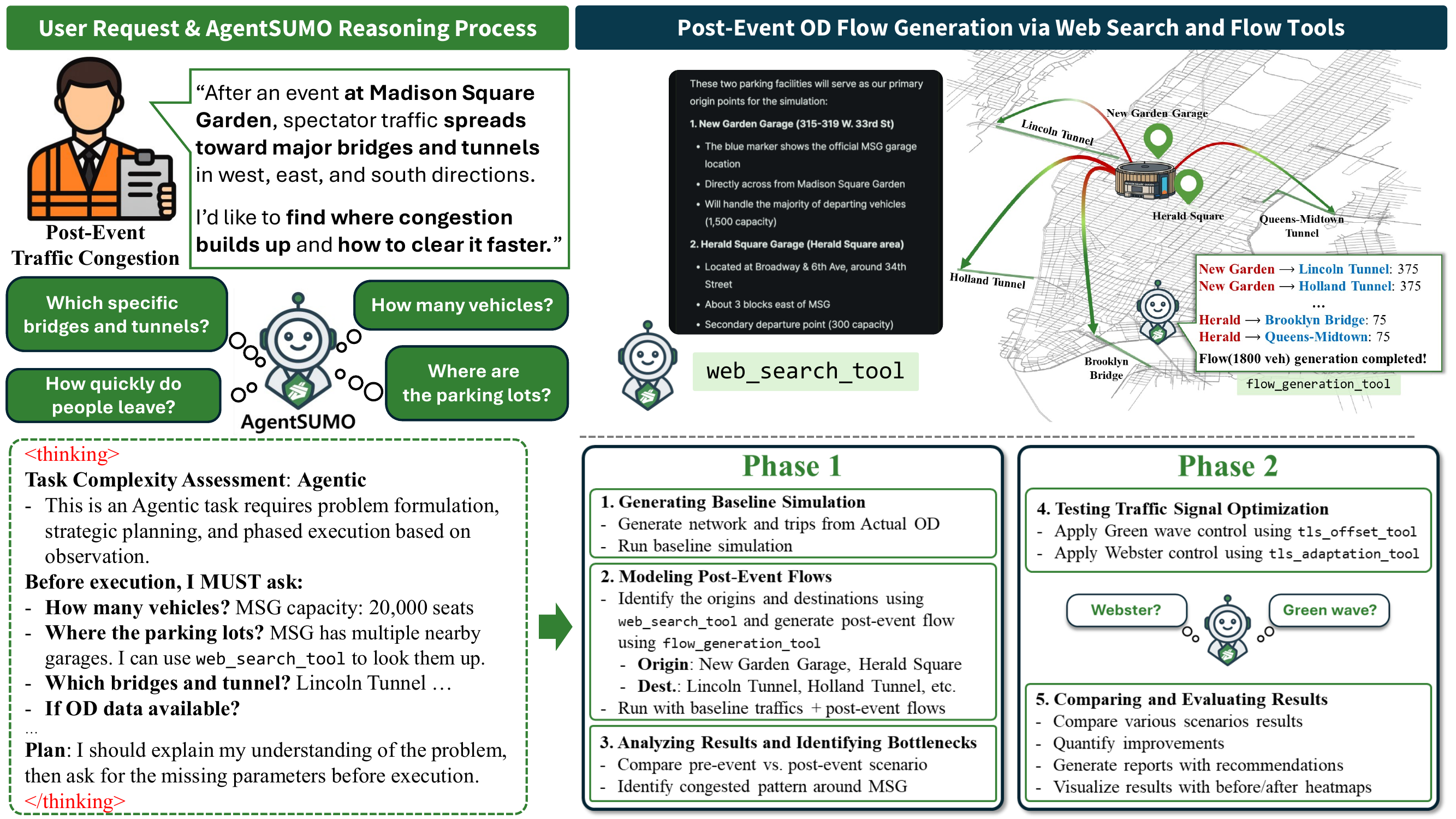
AgentSUMO workflow for the MSG post-event traffic management scenario. The IPP classifies the request as Agentic and the agent first asks clarification questions about the venue, parking origins, exits, and demand. In Phase 1 it generates the baseline, models the event flows with web_search_tool for parking and crossing lookups, and identifies the bottleneck around MSG. In Phase 2 it applies two signal-control policies through tls_offset_tool and tls_adaptation_tool and compares the four conditions.

Scenario design

Following the paper:

• Study area — Manhattan south of Central Park (64.3 km², 24 576 edges, 18 152 junctions).

• Background demand — 32 480 weekday-morning trips between 07:00 and 09:00 drawn from the publicly released NYC TLC yellow-taxi records. Each record’s pickup/dropoff coordinates form one OD pair.

• Event demand — 1 800 vehicles leaving MSG over a 30-minute window at the start of the simulation, distributed across two parking facilities and four major Manhattan crossings:

  • Origins — New Garden Garage (1 500 veh) on W. 33rd St and Herald Square Garage (300 veh).

  • Destinations — Lincoln Tunnel, Holland Tunnel, Queens-Midtown Tunnel, Brooklyn Bridge (450 veh each).

• Simulation duration — 3 hours so trips entering near the end of the surge can complete.

• Conditions —

  • Baseline — background demand only, default signal timings.

  • Post-Event — background + 1 800 event vehicles, default signals.

  • Green Wave — Post-Event + offset coordination via tls_offset_tool.

  • Webster — Post-Event + cycle-length adaptation via tls_adaptation_tool.

• Reporting levels — vehicle (restricted to the 1 800 event vehicles), edge (length-weighted speed and density on the MSG corridor along 7th, 8th, 9th Avenues and W. 28th–36th St — 423 edges, 23.7 km), and network (system-wide average travel time and peak halting vehicles).

Step 1 — Generate the Manhattan baseline

Build a baseline for Manhattan south of Central Park. Run a 3-hour morning
simulation between 07:00 and 09:00 using the NYC TLC taxi records I have
locally as the OD source.

The IPP classifies this as Simple because the parameters are all present once the OD source is provided. The agent runs the Scenario Generation pipeline (osm_extract → net_convert → trip_generate in Real OD mode (trip_type="real" — reads coordinate-based OD pairs from a CSV rather than synthesizing random trips) reading the TLC CSV → route_generate → sumo_runner) and ingests the run as simulation_id = "msg_baseline".

Step 2 — Add the MSG post-event surge

Paste:

After an event at Madison Square Garden, spectator traffic spreads toward
major bridges and tunnels in the west, east, and south directions. I'd
like to find where congestion builds up and how to clear it faster.

The IPP classifies this as Agentic — the request is open-ended (“find where congestion builds up and how to clear it faster”) and the response requires both planning across phases and external knowledge the network does not contain. The agent asks clarification questions about the venue capacity, the parking facilities, the per-origin vehicle counts, the crossings to target, and whether OD data is available, and proposes a two-phase plan. Once you confirm the plan:

1. The agent calls web_search_tool to retrieve approximate coordinates for the two MSG parking facilities and the four crossings.

2. It calls validate_od_coordinates_tool to confirm each coordinate falls inside the network and to resolve the nearest valid edge.

3. It calls flow_generation_tool once per origin-destination pair (2 origins × 4 destinations = 8 flows), each appending a flow to the route file with vehs_per_hour chosen so the total over 30 minutes matches the 1 800-vehicle budget.

4. It re-runs sumo_runner with the combined demand and ingests the result as simulation_id = "msg_post_event".

Step 3 — Apply the Green Wave signal policy

Apply Green Wave coordination on the corridors around MSG and rerun the
post-event scenario. Save it as "msg_green_wave".

The agent invokes tls_offset_tool, which wraps SUMO’s tlsCoordinator.py. The tool writes a supplementary XML file containing offset adjustments for the affected intersections. The agent passes this file to sumo_runner via additional_files against the same Post-Event demand, then ingests the run.

Step 4 — Apply the Webster signal policy

Now try Webster-style cycle adaptation on the same corridors. Save it as
"msg_webster".

The agent invokes tls_adaptation_tool, which wraps SUMO’s tlsCycleAdaptation.py. The procedure mirrors Step 3: write a supplementary XML with adapted cycle lengths, run the simulation against the Post-Event demand, ingest the result.

Step 5 — Compare the four conditions

Paste:

Compare the four conditions across three levels:
1. Vehicle level — average duration and reroute count for the 1,800 event
   vehicles only.
2. Edge level — length-weighted speed and density on the MSG corridor
   (7th, 8th, 9th Avenues + W. 28th to 36th St).
3. Network level — average travel time and peak halting vehicles
   system-wide.

The agent identifies the 1 800 event vehicles by the flow_-prefixed trip IDs generated in Step 2, length-weights the corridor metrics across the 23.7 km / 423 edges, and aggregates the network metrics over all 3 hours. The paper observed the following pattern (Table 7):

Level	Metric	Baseline	Post-Event	Green Wave	Webster
Vehicle	Avg. duration (s)	—	987	726	935
Vehicle	Avg. reroute count	—	1.468	1.314	1.464
Edge	Avg. speed (m/s)	7.56	7.38	8.35	6.81
Edge	Avg. density (veh/km)	7.51	9.15	5.81	9.32
Network	Avg. travel time (s)	574.7	588.0	361.4	505.3
Network	Peak halting vehicles	2 872	3 072	955	2 027

Three patterns emerge. First, the network absorbs the surge well overall (+2 % travel time over baseline), but the corridor signature is sharp (+22 % density, −2 % speed) — the network mean hides the local redistribution that operators most care about. Second, Green Wave improves all three levels at once: corridor speed rises 10 % above baseline, corridor density falls 23 %, and peak halting drops 67 % network-wide. Third, Webster improves the network mean (travel time −12 %, peak halting −29 %) but raises corridor density to 24 % above baseline — the largest of any condition. Webster improves the system mean while shifting congestion onto the corridor most exposed to the event.

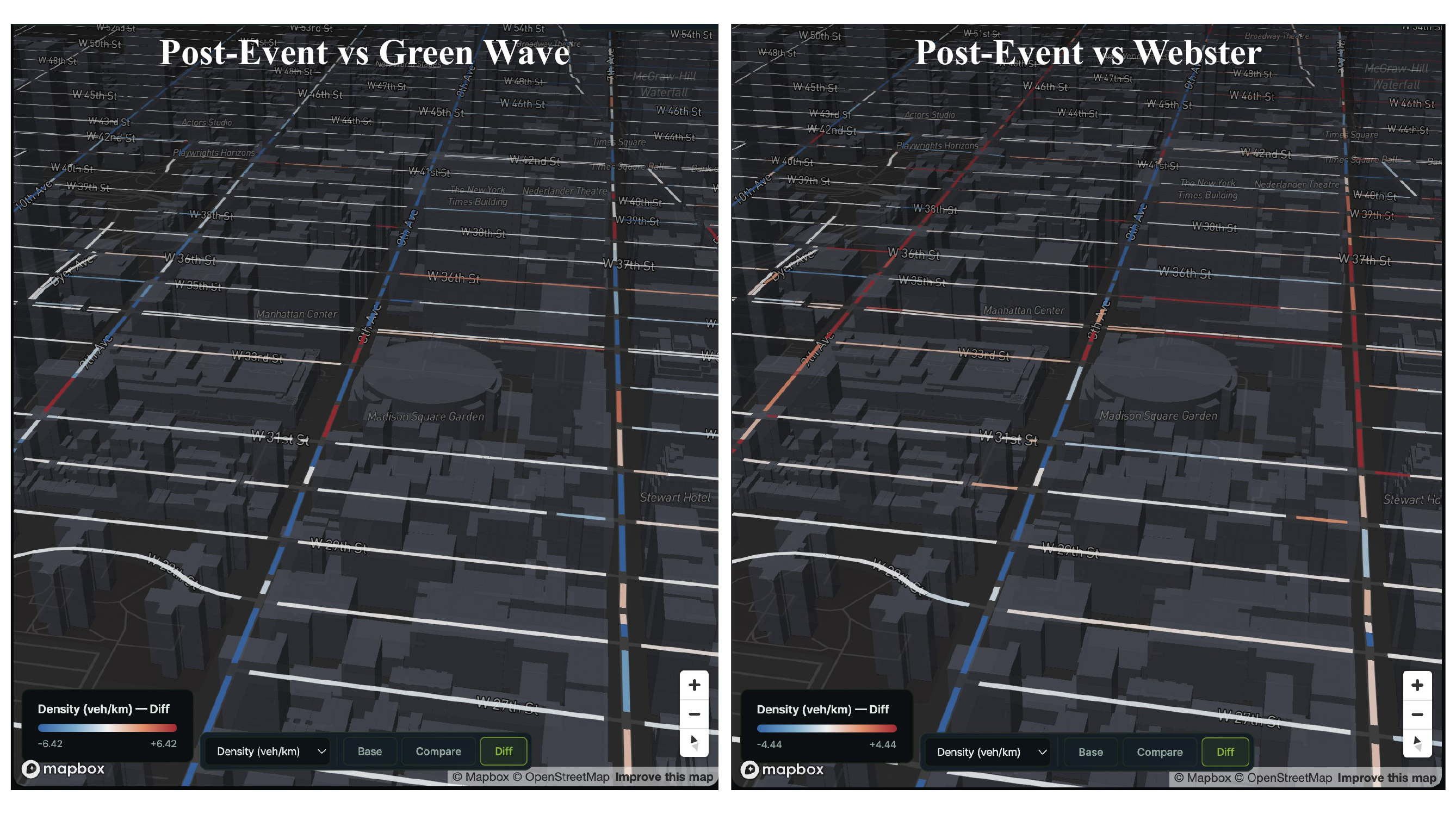
Difference heatmap of per-edge density between Post-Event and each signal policy, rendered on the AgentSUMO web interface’s 3D Mapbox base. Left: Post-Event vs Green Wave — avenues near MSG shift consistently toward blue, indicating reduced density. Right: Post-Event vs Webster — the effect is weaker and mixed, with some segments still blue but others shifting toward red.

Step 6 — Generate a report

Generate an HTML report comparing the baseline, the post-event surge,
Green Wave, and Webster.

The agent invokes simulation_report_tool, which writes a self-contained HTML report with the four-way KPI comparison, the top congested roads under each condition, and an inline SVG of the study area with the MSG corridor highlighted.

What you’ve practiced

• An Agentic task driven through the IPP — the agent formulated the problem from an open-ended goal, asked the right clarification questions, and decomposed the work into two phases.

• web_search_tool as a reasoning aid — the agent grounded scenario parameters in real-world facts (venue capacity, parking locations, Manhattan crossings) the network alone could not supply.

• Coordinate validation before flow generation — the agent verified each origin and destination resolved to a valid edge before committing to the OD plan.

• Trade-offs across reporting levels — the comparison surfaced a network-vs-corridor trade-off (Webster) that single aggregate metrics would obscure.

• Difference heatmaps as the spatial counterpart of the cross-scenario KPI table.

See also

• The Seoul Lane-Closure Timing tutorial for the Complex case with structured timing alternatives.

• The AgentSUMO MCP Server reference for every tool the agent invoked.

• The Schema page for the column-level structure of the queries used in Step 5.