Tutorial — Seoul Lane-Closure Timing#
This walkthrough reproduces the Seoul construction-timing case study from the paper (Section 5.3.1): a planner is choosing when to schedule a temporary lane closure on Teheran-ro during the morning commute and asks AgentSUMO to compare two candidate windows.
The decision is a Complex task: a clear policy intervention (one-lane closure on a known corridor) with an underspecified parameter (the timing window). The agent’s job is to resolve that ambiguity through dialogue, construct a baseline and the two candidate scenarios, and present a comparison that supports the scheduling decision.
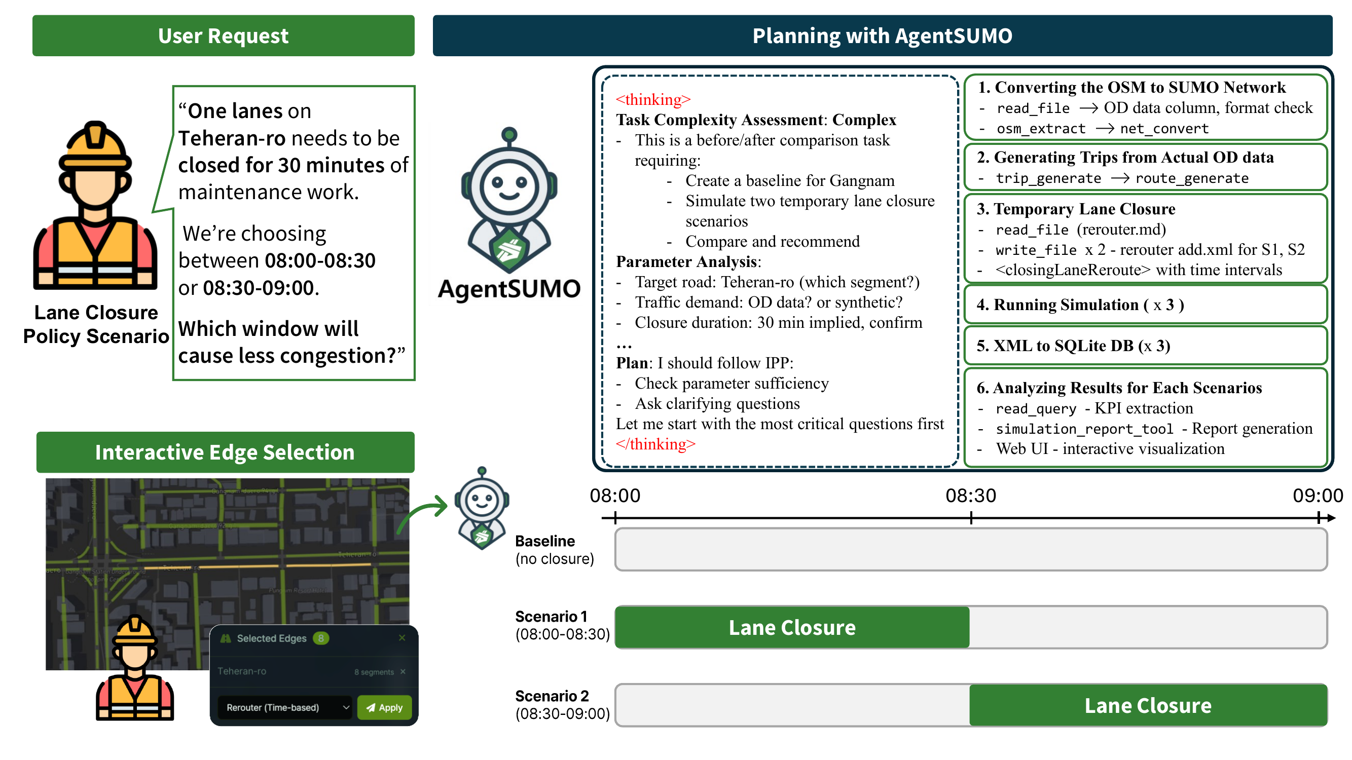
AgentSUMO workflow for the Teheran-ro construction time-window scenario. The IPP classifies the request as Complex and elicits the target segment, demand source, and closure duration. The user marks the construction zone on the rendered network through edge selection, and the agent then drives the tool-call sequence across baseline and the two timed-closure scenarios.#
Scenario design#
Following the paper:
Study area — Gangnam district, Seoul (53.8 km², 15 731 edges, 5 697 junctions).
Demand — 6 200 morning-commute trips between 07:00 and 09:00, derived from anonymized taxi-trajectory records.[1] In this tutorial we substitute RandomOD demand at medium intensity for reproducibility.
Simulation duration — 3 hours.
Intervention — close one lane along eight consecutive edges of Teheran-ro (≈ 376 m corridor) for a single 30-minute window.
Scenarios —
Baseline — no closure.
S₁ — closure during 08:00–08:30 (peak-overlapping).
S₂ — closure during 08:30–09:00 (post-peak).
Reporting levels — vehicle (time loss, reroute count), edge (length-weighted speed and density on the closed corridor), and network (average travel time, peak halting vehicles).
The Korean 5030 speed-limit policy is applied throughout: 50 km/h on arterials, 30 km/h on residential streets.
Step 1 — Generate the baseline#
Open the web interface and paste:
Build a baseline for the Gangnam district around Gangnam Station with a
1.5 km radius. Run a 3-hour morning-commute simulation between 07:00 and
09:00 with medium traffic.
The IPP classifies the request as Simple because every parameter is present. The agent confirms the inferred network bounds and runs the Scenario Generation pipeline:
osm_extract→net_convert— build the SUMO network for the Gangnam bounding box.trip_generate→route_generate— synthesize morning-commute demand and assign shortest-path routes.sumo_runner— execute the 3-hour simulation and capturetripinfo.xml,edgeData.xml,edgeData_emission.xml, plus the vehicle-position replay JSON.xml_to_sqlite_tool— ingest the results undersimulation_id = "baseline"so the comparison in Step 4 can use SQL.
Step 2 — Apply S₁ (peak-overlapping closure, 08:00–08:30)#
Paste:
One lane on Teheran-ro needs to be closed for 30 minutes of maintenance
work. Test the impact of closing it during 08:00 - 08:30. Save it as
"teheran_S1_peak_overlap".
The IPP classifies this as Complex: a clear intervention type but with multiple targets (which lane segment) and explicit timing. Following the clarify-before-execute step:
The agent calls
analyze_road_details_toolwithtarget_road_name = "Teheran-ro"and the Gangnam-Station reference point to enumerate the candidate edges.It calls
visualize_policy_target_toolto render the eight-segment construction zone over the network and asks you to confirm.Because the closure is temporal rather than permanent, the agent does not modify the network. Instead it follows the guide-based path of the Filesystem MCP Server, reading
rerouter.mdto recall the schema and writing a*.add.xmlfile with a<closingLaneReroute>element scoped to the 08:00–08:30 window.It re-runs
sumo_runneragainst the same baseline network and route file with the newadditional_filespassed through. Trips and routes are reused because edge IDs are preserved.The result is ingested as
simulation_id = "teheran_S1_peak_overlap".
Tip
You can mark the eight construction segments graphically: enter edge-selection mode in the map toolbar, click the corridor, choose Rerouter (Time-based), set the closure window, and submit. The agent receives the structured marker and produces an identical rerouter file.
Step 3 — Apply S₂ (post-peak closure, 08:30–09:00)#
Paste:
Now test the same closure shifted 30 minutes later — 08:30 to 09:00.
Save it as "teheran_S2_post_peak".
Because the network and route file are unchanged, the agent skips the
target-segment dialogue (it remembers the eight edges from Step 2 through
session state) and proceeds directly
to writing a new rerouter file with the shifted window, running the
simulation, and ingesting it as
simulation_id = "teheran_S2_post_peak".
Step 4 — Compare the three scenarios#
Paste:
Compare the baseline, S1, and S2 across three levels:
1. Vehicle level — average time loss and reroute count.
2. Edge level — length-weighted speed and density on the closed corridor.
3. Network level — average travel time and peak halting vehicles.
The agent issues SQL queries against the SQLite database. Edge-level metrics are length-weighted across the 376 m corridor to avoid bias from short segments, and the network-level metrics aggregate over all 3 hours of simulation. The paper observed the following pattern across the same three levels (Table 6):
Level |
Metric |
Baseline |
S₁ (peak overlap) |
S₂ (post-peak) |
|---|---|---|---|---|
Vehicle |
Avg. time loss (s) |
94.4 |
136.1 (+44 %) |
109.8 (+16 %) |
Vehicle |
Avg. reroute count |
0.105 |
0.124 (+18 %) |
0.108 (+3 %) |
Edge |
Avg. speed (m/s) |
11.4 |
8.1 (−28 %) |
8.4 (−26 %) |
Edge |
Avg. density (veh/km) |
5.2 |
10.3 (+98 %) |
8.6 (+65 %) |
Network |
Avg. travel time (s) |
251.1 |
261.1 (+4 %) |
255.7 (+2 %) |
Network |
Peak halting vehicles |
125 |
216 (+73 %) |
195 (+56 %) |
S₁ disrupts traffic more than S₂ at every level, and the gap widens as the scope moves from the corridor to the network. Both windows reduce corridor speed similarly (28 % vs 26 %), but the density response diverges (+98 % under S₁ vs +65 % under S₂) — under S₁ more drivers meet queues severe enough to trigger rerouting, and peak halting rises 73 % network-wide.
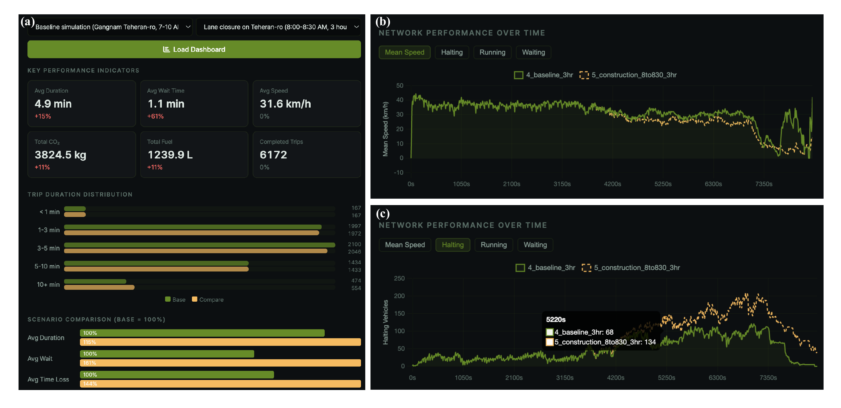
Comparative dashboard for any two selected runs, shown here for the baseline and the peak-overlapping closure (S₁). KPI cards quantify the change between the pair; the time-series panels add a temporal profile, with halting vehicles rising through the closure window and mean speed declining over the same interval.#
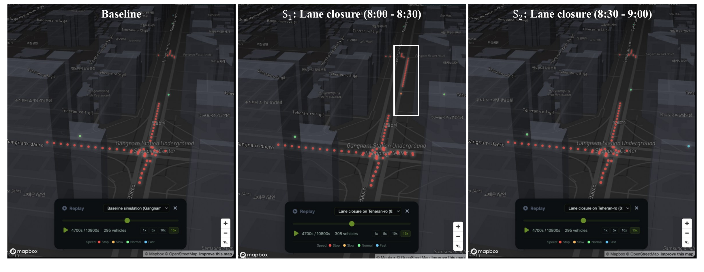
Simulation replay of the three scenarios at t ≈ 4 700 s (08:18), well within the S₁ window. Left: Baseline. Center: S₁, where a stationary queue forms on the closed Teheran-ro segment. Right: S₂, whose closure window has not yet begun, so it remains free-flowing like the baseline.#
Step 5 — Generate a report#
For sharing with stakeholders:
Generate an HTML report comparing the baseline, S1, and S2.
The agent invokes simulation_report_tool, which queries the SQLite
database for all three simulation_ids, computes KPIs, ranks the most
congested roads via length-weighted average density, renders an inline
SVG of the study-area network with the Teheran-ro construction zone
highlighted, and writes a self-contained HTML file to
outputs/reports/.
What you’ve practiced#
A Complex task driven through the Interactive Planning Protocol — the agent resolved the ambiguous timing parameter through dialogue and confirmed the construction zone visually before proceeding.
A temporal policy intervention using the guide-based Filesystem workflow, where the agent reads
rerouter.mdand writes a supplementary XML file rather than editing the network.Session state continuity — Step 3 reused the construction segments established in Step 2 without re-prompting.
A three-level comparison through SQL on the structured database, surfacing redistribution that vehicle-level metrics alone would miss.
See also
The Manhattan Post-Event Management tutorial for the more open-ended Agentic case.
The AgentSUMO MCP Server reference for every tool the agent invoked along the way.
The Schema page for the column-level structure of the queries used in Step 4.